The competition solution workflow goes through seven stages described in the Data Science Solutions book.
1.Question or problem definition.
2.Acquire training and testing data.
3.Wrangle, prepare, cleanse the data.
4.Analyze, identify patterns, and explore the data.
5.Model, predict and solve the problem.
6.Visualize, report, and present the problem solving steps and final solution.
7.Supply or submit the results.
The workflow indicates general sequence of how each stage may follow the other. However there are use cases with exceptions.
a.We may combine mulitple workflow stages. We may analyze by visualizing data.
b.Perform a stage earlier than indicated. We may analyze data before and after wrangling.
c.Perform a stage multiple times in our workflow. Visualize stage may be used multiple times.
d.Drop a stage altogether. We may not need supply stage to productize or service enable our dataset for a competition.
Question and problem definition
Competition sites like Kaggle define the problem to solve or questions to ask while providing the datasets for training your data science model and testing the model results against a test dataset. The question or problem definition for Titanic Survival competition is described here at Kaggle.
Knowing from a training set of samples listing passengers who survived or did not survive the Titanic disaster, can our model determine based on a given test dataset not containing the survival information, if these passengers in the test dataset survived or not.
We may also want to develop some early understanding about the domain of our problem. This is described on the Kaggle competition description page here. Here are the highlights to note.
On April 15, 1912, during her maiden voyage, the Titanic sank after colliding with an iceberg, killing 1502 out of 2224 passengers and crew. Translated 32% survival rate.
One of the reasons that the shipwreck led to such loss of life was that there were not enough lifeboats for the passengers and crew.
Although there was some element of luck involved in surviving the sinking, some groups of people were more likely to survive than others, such as women, children, and the upper-class.
Workflow goals
The data science solutions workflow solves for seven major goals.
Classifying. We may want to classify or categorize our samples. We may also want to understand the implications or correlation of different classes with our solution goal.
Correlating. One can approach the problem based on available features within the training dataset. Which features within the dataset contribute significantly to our solution goal? Statistically speaking is there a correlation among a feature and solution goal? As the feature values change does the solution state change as well, and visa-versa? This can be tested both for numerical and categorical features in the given dataset. We may also want to determine correlation among features other than survival for subsequent goals and workflow stages. Correlating certain features may help in creating, completing, or correcting features.
Converting. For modeling stage, one needs to prepare the data. Depending on the choice of model algorithm one may require all features to be converted to numerical equivalent values. So for instance converting text categorical values to numeric values.
Completing. Data preparation may also require us to estimate any missing values within a feature. Model algorithms may work best when there are no missing values.
Correcting. We may also analyze the given training dataset for errors or possibly innacurate values within features and try to corrent these values or exclude the samples containing the errors. One way to do this is to detect any outliers among our samples or features. We may also completely discard a feature if it is not contribting to the analysis or may significantly skew the results.
Creating. Can we create new features based on an existing feature or a set of features, such that the new feature follows the correlation, conversion, completeness goals.
Charting. How to select the right visualization plots and charts depending on nature of the data and the solution goals.
1 | #数据分析 |
1 | #读取数据 |
1 | ['PassengerId' 'Survived' 'Pclass' 'Name' 'Sex' 'Age' 'SibSp' 'Parch' |
1 | train_df.head(2) |
1 | test_df.head(2) |
1 | train_df.tail() |
1 | train_df.info() |
1 | <class 'pandas.core.frame.DataFrame'> |
1 | train_df.describe() |
1 | train_df.describe(include=['O']) |
类别、序列、离散特征的分析
1 | train_df[['Pclass','Survived']].groupby(['Pclass'],as_index=False).mean().sort_values(by='Survived',ascending=False) |
1 | train_df[["SibSp", "Survived"]].groupby(['SibSp'], as_index=False).mean().sort_values(by='Survived', ascending=False) |
1 | train_df[["Parch", "Survived"]].groupby(['Parch'], as_index=False).mean().sort_values(by='Survived', ascending=False |
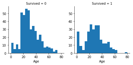
可视化数值特征
1 | g=sns.FacetGrid(train_df,col='Survived') |
1 | <seaborn.axisgrid.FacetGrid at 0xc574f60> |
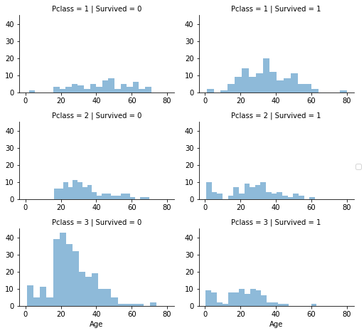
1 | grid=sns.FacetGrid(train_df,col='Survived',row='Pclass',size=2.2,aspect=1.6) |
1 | <seaborn.axisgrid.FacetGrid at 0xc619278> |
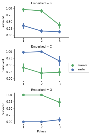
1 | grid=sns.FacetGrid(train_df,row='Embarked',size=2.2,aspect=1.6) |
1 | <seaborn.axisgrid.FacetGrid at 0xcd8f358> |
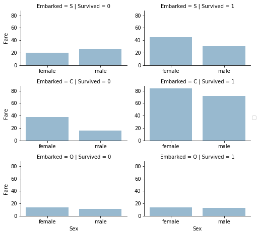
1 | grid=sns.FacetGrid(train_df,row='Embarked',col='Survived',size=2.2,aspect=1.6) |
1 | <seaborn.axisgrid.FacetGrid at 0xcf12f60> |
去除特征
1 | print("Before",train_df.shape,test_df.shape,combine[0].shape,combine[1].shape) |
1 | Before (891, 12) (418, 11) (891, 12) (418, 11) |
1 | train_df=train_df.drop(['Ticket','Cabin'],axis=1) |
1 | After (891, 10) (418, 9) (891, 10) (418, 9) |
1 | train_df.info() |
1 | <class 'pandas.core.frame.DataFrame'> |
1 | train_df.head(1) |
creating new feature extracting from existing
1 | for dataset in combine: |
1 | dataset.shape |
1 | (418, 10) |
1 | pd.crosstab(train_df['Title'],train_df['Sex'] |
1 | #replace many titles with a more common name or classify them as Rare |
1 | #将类别特征转换成数值特征 |
1 | train_df.head() |
1 | test_df.head(1) |
1 | #删除训练集和测试集中的Name特征,删除训练集中的name特征 |
1 | combine=[train_df,test_df] |
1 | ((891, 9), (418, 9)) |
1 | for dataset in combine: |
1 | train_df.info() |
1 | <class 'pandas.core.frame.DataFrame'> |
补全缺失值(数值连续特征)
1.生成随机数[mean,std]
2.通过相关特征预测预测缺失值,如年龄,性别,pclass特征,可以根据相同性别,pclass的样本的中位数预测年龄
3.前两种方法组合,用相关特征的样本的均值和方差之间进行随机生成数据
第1,2种方法都包含随机性,一般选择第二种
1 | grid=sns.FacetGrid(train_df,row='Pclass',col='Sex',size=2.2,aspect=1.6) |
1 | <seaborn.axisgrid.FacetGrid at 0xe211f28> |
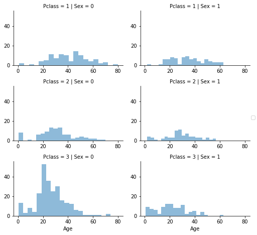
1 | guess_ages=np.zeros((2,3)) |
1 | array([[ 0., 0., 0.], |
1 | for dataset in combine: |
1 | #let us create Age bands and determine correlations with Survived |
1 | #let us replace Age with ordinals based on these bands |
1 | #we can not removet the AgeBand feature |
1 | #create new feature combining existing features |
1 | #we can create another feature called IsAlone |
1 | #let us drop Parch,SibSp,and FamilySize features in faver of IsAlone |
1 | train_df.head() |
1 | #we can also create an artificial feature combining Pclass and Age |
1 | #completing a categorical feature |
1 | <class 'pandas.core.frame.DataFrame'> |
1 | #Embarked feature takes S,Q,C values based on port of embarkation. |
1 | 'S' |
1 | for dataset in combine: |
1 | #Converting categorical feature to numeric |
1 | #Quick completing and converting a numeric feature |
1 | test_df.info() |
1 | <class 'pandas.core.frame.DataFrame'> |
1 | ''' |
1 | #we can not create FareBand |
1 | #convert the Fare feature to ordinal values based on the FareBand |
1 | #And the test dataset |
Model,Predict and solve
接下来我们 要训练一个模型进行预测。一共有60+预测模型以供我们选择,我们必须理解问题的类型,将解决方案缩小到几个可选的模型中去。我们的问题是一个分类和回归的问题,我们想要确定输出(survived or not)和特征变量之间的关系。我们将要执行一种监督学习的模型,在训练过程中会给定数据。在监督学习和分类回归条件下,我们将模型缩小到一下几种:
1.逻辑回归
2.KNN
3.支持向量机
4.贝叶斯
5.决策树
6.随机森林
7.感知机
8.人工神经网络
9.RVM or Relevance Vector Machine
1 | X_train=train_df.drop("Survived",axis=1) |
1 | ((891, 8), (891,), (418, 8)) |
1 | train_df.head() |
1 | test_df.head() |
1.Logistic Regression
1 | logreg=LogisticRegression() |
1 | 80.579999999999998 |
1 | logreg = LogisticRegression() |
1 | 80.579999999999998 |
‘’’
We can use Logistic Regression to validate our assumptions and decisions for feature creating and completing goals.
This can be done by calculating the coefficient of the features in the decision function.
Positive coefficients increase the log-odds of the response (and thus increase the probability),
and negative coefficients decrease the log-odds of the response (and thus decrease the probability).
1.Sex is highest positivie coefficient, implying as the Sex value increases (male: 0 to female: 1), the probability of Survived=1 increases the most.
2.Inversely as Pclass increases, probability of Survived=1 decreases the most.
3.This way Age*Class is a good artificial feature to model as it has second highest negative correlation with Survived.
4.So is Title as second highest positive correlation.
‘’’
1 | coeff_df=pd.DataFrame(train_df.columns.delete(0)) |
SVM
SVM training algorithm builds a model that assigns new test samples to one category or the other, making it a non-probabilistic binary linear classifier.
Note that the model generates a confidence score which is higher than Logistics Regression model
1 | svc=SVC() |
1 | 84.290000000000006 |
KNN
In pattern recognition, the k-Nearest Neighbors algorithm (or k-NN for short) is a non-parametric method used for classification and regression. A sample is classified by a majority vote of its neighbors, with the sample being assigned to the class most common among its k nearest neighbors (k is a positive integer, typically small). If k = 1, then the object is simply assigned to the class of that single nearest neighbor.
KNN confidence score is better than Logistics Regression and not worse than SVM.
1 | knn=KNeighborsClassifier(n_neighbors=3) |
1 | 84.849999999999994 |
Bayes
In machine learning, naive Bayes classifiers are a family of simple probabilistic classifiers based on applying Bayes’ theorem with strong (naive) independence assumptions between the features. Naive Bayes classifiers are highly scalable, requiring a number of parameters linear in the number of variables (features) in a learning problem.
The model generated confidence score is the lowest among the models evaluated so far.
1 | #Gaussian Naive Bayes |
1 | 71.379999999999995 |
Perceptron
The perceptron is an algorithm for supervised learning of binary classifiers (functions that can decide whether an input, represented by a vector of numbers, belongs to some specific class or not). It is a type of linear classifier, i.e. a classification algorithm that makes its predictions based on a linear predictor function combining a set of weights with the feature vector. The algorithm allows for online learning, in that it processes elements in the training set one at a time.
1 | perceptron=Perceptron() |
1 | D:\noSystem\software\Anaconda3\lib\site-packages\sklearn\linear_model\stochastic_gradient.py:128: FutureWarning: max_iter and tol parameters have been added in <class 'sklearn.linear_model.perceptron.Perceptron'> in 0.19. If both are left unset, they default to max_iter=5 and tol=None. If tol is not None, max_iter defaults to max_iter=1000. From 0.21, default max_iter will be 1000, and default tol will be 1e-3. |
1 | 79.569999999999993 |
Linear SVC
1 | linear_svc=LinearSVC() |
1 | 80.129999999999995 |
Stochastic Gradient Descent
1 | sgd=SGDClassifier() |
1 | D:\noSystem\software\Anaconda3\lib\site-packages\sklearn\linear_model\stochastic_gradient.py:128: FutureWarning: max_iter and tol parameters have been added in <class 'sklearn.linear_model.stochastic_gradient.SGDClassifier'> in 0.19. If both are left unset, they default to max_iter=5 and tol=None. If tol is not None, max_iter defaults to max_iter=1000. From 0.21, default max_iter will be 1000, and default tol will be 1e-3. |
Decision Tree
This model uses a decision tree as a predictive model which maps features (tree branches) to conclusions about the target value (tree leaves). Tree models where the target variable can take a finite set of values are called classification trees; in these tree structures, leaves represent class labels and branches represent conjunctions of features that lead to those class labels. Decision trees where the target variable can take continuous values (typically real numbers) are called regression trees.
The model confidence score is the highest among models evaluated so far.
1 | decision_tree=DecisionTreeClassifier() |
1 | 87.209999999999994 |
Random Forest
The next model Random Forests is one of the most popular. Random forests or random decision forests are an ensemble learning method for classification, regression and other tasks, that operate by constructing a multitude of decision trees (n_estimators=100) at training time and outputting the class that is the mode of the classes (classification) or mean prediction (regression) of the individual trees.
The model confidence score is the highest among models evaluated so far. We decide to use this model’s output (Y_pred) for creating our competition submission of results.
1 | random_forest=RandomForestClassifier(n_estimators=100) |
1 | 87.209999999999994 |
模型评估
We can now rank our evaluation of all the models to choose the best one for our problem. While both Decision Tree and Random Forest score the same, we choose to use Random Forest as they correct for decision trees’ habit of overfitting to their training set.
1 | models=pd.DataFrame({ |
1 | submission=pd.DataFrame({ |
Our submission to the competition site Kaggle results in scoring 3,883 of 6,082 competition entries. This result is indicative while the competition is running. This result only accounts for part of the submission dataset. Not bad for our first attempt. Any suggestions to improve our score are most welcome.